Distance analysis

Minimum-distance benchmark

A degree-distribution benchmark derived from the average weight enumerator of regular LDPC-type ensembles.

Scope. This is a typical-relative-distance benchmark for a degree distribution. It is not a rigorous minimum-distance lower bound for any particular finite-length CSS code.

Benchmark figure

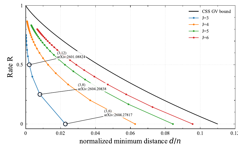
Minimum-distance benchmark for regular degree distributions — The horizontal axis is normalized distance (d/n), and the vertical axis is rate (R). The black curve is the CSS Gilbert–Varshamov bound. Colored curves show regular LDPC-type benchmarks for column weights (J=3,4,5,6). Circled points mark the ((3,12)), ((3,8)), and ((3,6)) finite-length design choices used in related constructions.

Definition

For relative weight δ, write the expected number of codewords in a ((J,L))-regular random LDPC-type ensemble as

\[\mathbb{E}A_{\delta n}\doteq \exp\!\left(n\gamma_{J,L}(\delta)\right).\]

The plotted benchmark is the first positive δ satisfying γ_J,L(δ)=0, where

\[\gamma_{J,L}(\delta)=h(\delta)+\frac{J}{L}\log P_L(x)-J\delta\log x-Jh(\delta),\qquad P_L(x)=\frac{(1+x)^L+(1-x)^L}{2},\]

and (x) is the positive saddle-point solution of

\[\frac{xP_L'(x)}{P_L(x)}=L\delta.\]

For a fixed column weight (J), varying (L) gives the CSS design rate (R=1-2J/L). The black CSS GV curve is (R=1-2h_2(\delta)).

How to interpret it

Use the curves to compare degree distributions before committing to a finite-length construction.
Do not read a plotted point as an exact distance or as a certificate for a particular code.
For explicit finite-length evidence, use the live catalog, parameter files, and distance-witness notes.

Finite-length evidence

Live code catalog

Current code parameters, lower-bound status, and method-specific upper bounds.

Open catalog →

Upper-bound definitions

Definitions and interpretation of latent, block, quotient, CRT, direct-CSS, and decoder-failure witnesses.

Read the notes →